Xoilac TV trực tiếp bóng đá mọi giải đấu hàng đầu thế giới và Việt Nam hoàn toàn miễn phí. Đặc biệt, Xôi Lạc TV TTBD cam kết đảm bảo chất lượng hình ảnh và âm thanh sắc nét suốt 90 phút, bạn sẽ không bỏ lỡ bất kỳ khoảnh khắc xem bóng đá trực tuyến đỉnh cao trên sân cỏ.
Xoilac là trang web phát sóng trực tiếp bóng đá hôm nay miễn phí với chất lượng cao, là địa chỉ xem bóng đá online phổ biến hàng đầu tại Việt Nam. Cung cấp đầy đủ link tructiepbongda các trận đấu từ cả trong và ngoài nước, mang đến cho bạn trải nghiệm xem bóng đá tốt nhất.

Hãy truy cập ngay vào Xoilactv xem bóng đá để có link xem bóng đá uy tín nhất, đảm bảo bạn sẽ hài lòng với trải nghiệm xem trực tuyến của mình. Không còn lo lắng về việc bỏ lỡ những trận đấu hấp dẫn, hãy đồng hành cùng chúng tôi để theo dõi mọi diễn biến trong thế giới bóng đá hiện đại!
Các BLV chuyên nghiệp hiện có trên XoilacTV: King, Mát Gai, Củ Cải, AK47, Cá, Fanta, Đốm, Rickhanter, Tạ Biên Giới, Rio, Deco, Singer, Ram , Tommy, Sùng A Múp, Công Lý, Măng Cục, Phi Hành…
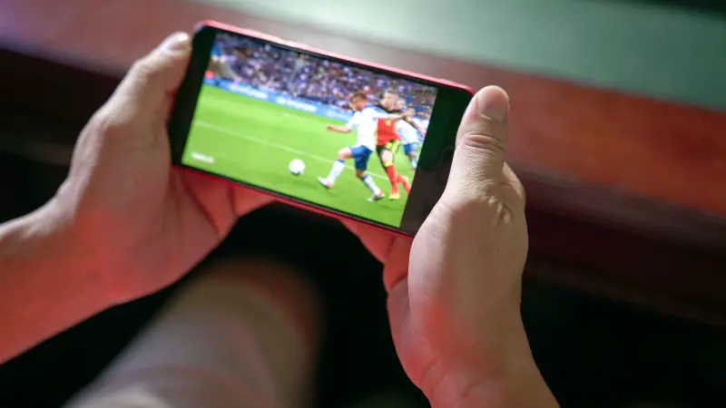
Thời đại công nghệ số đang phát triển mạnh mẽ và người ta ngày càng ưa chuộng việc xem trực tiếp bóng đá qua các thiết bị như điện thoại di động, máy tính, thay vì truyền hình như trước đây. Để đảm bảo trải nghiệm xem bóng đá tốt nhất, việc lựa chọn vào một trang web uy tín là điều quan trọng hàng đầu.

Tại Việt Nam, lựa chọn các trang web đáng tin cậy để xem trực tiếp bóng đá không nhiều. Đó là lý do Xoilac ra đời với mục tiêu cung cấp cho người hâm mộ một địa chỉ xem bóng đá chất lượng cao. Bạn có thể tin tưởng vào Xoilac để có trải nghiệm xem trực tiếp bóng đá với chất lượng hình ảnh và âm thanh tốt nhất.
Xoilac TV có dàn đội ngũ hỗ trợ phía sau là các chuyên gia bóng đá hàng đầu tại Việt Nam, kèm theo đó là các kỹ thuật viên IT chuyên nghiệp. Nhờ sự kết hợp này, chúng tôi đã phát triển nhanh chóng, áp dụng công nghệ mới nhất vào cơ sở hạ tầng của mình. Trong thời gian ngắn, Xoilac đã thu hút một lượng người xem đáng kể.
Mục tiêu phát triển của chúng tôi là phục vụ người xem trải nghiệm tốt nhất. Bạn chỉ cần truy cập vào Xoilac để lấy đường link xem trực tiếp bóng đá nhanh chóng. Hệ thống link xem trực tiếp bóng đá của chúng tôi bao gồm Champion League, Ngoại Hạng Anh, La Liga, Bundesliga, Serie A, Ligue 1, Cúp C2, Euro 2024, World Cup 2026, Copa America, v.v. Với những đường link này, bạn sẽ được trải nghiệm trận đấu chất lượng siêu nét, hấp dẫn và có BLV tiếng việt rõ ràng.
Ngoài phát sóng bóng đá miễn phí với chất lượng cao, Xoilac còn cung cấp thông tin bổ ích như sự kiện, tin tức bóng đá, kết quả bóng đá hôm nay, lịch thi đấu, bảng xếp hạng, kèo nhà cái của các giải đấu hàng đầu. Tất cả thông tin này được liên tục cập nhật một cách chính xác nhất.

Sứ mệnh là nơi dành cho người hâm mộ xem trực tiếp bóng đá hàng đầu tại Việt Nam, Xoilac không ngừng phát triển và nâng cấp để mang lại trải nghiệm xem bóng đá trực tuyến tốt nhất cho mọi người.
Khi bạn truy cập trang web phát sóng bóng đá trực tiếp của Xoilac TV, bạn sẽ trải qua một trải nghiệm đầy bất ngờ. Chúng tôi không chỉ cung cấp link trực tiếp bóng đá cho các giải đấu lớn như Ngoại Hạng Anh, Champion League, La Liga, Bundesliga,Serie A, Ligue 1, World Cup, Euro, Copa America mà còn cập nhật đầy đủ link xem các giải bóng đá trong nước và khu vực như Sea Games, AFF Cup, U23 Châu Á, V-League và nhiều giải đấu khác.
Đặc biệt, XoilacTV không chỉ giới hạn trong việc cung cấp link xem trực tiếp, mà còn đảm bảo cập nhật thông tin bóng đá liên tục. Tại đây, bạn có thể dễ dàng theo dõi mọi thông tin mới nhất về bóng đá trong và ngoài nước, từ kết quả bóng đá (KQBD), lịch thi đấu, keonhacai, bảng xếp hạng đến những tin tức bóng đá nổi bật hàng ngày.
Chúng tôi cam kết mang đến cho người xem không chỉ những trận đấu hấp dẫn mà còn một nguồn thông tin đáng tin cậy và đầy đủ, làm hài lòng mọi người hâm mộ bóng đá. Hãy trải nghiệm ngay trên Xoilac để không chỉ xem bóng đá mà còn cập nhật đầy đủ thông tin bóng đá mọi lúc, mọi nơi.
Hiện tại, sự quan tâm của đa số người hâm mộ đổ vào việc xem các trận đấu của những CLB hàng đầu như Man City, Liverpool, Man United, Real Madrid, Barcelona, Bayern Munich, Juventus, và cả những đội tuyển quốc gia nổi tiếng như Pháp, Argentina, Anh, Bồ Đào Nha, Đức, Tây Ban Nha, Brazil, Croatia, v.v. Chúng tôi hiểu điều này và đáp ứng nhanh chóng bằng cách cập nhật đầy đủ và chất lượng link xem trực tiếp cho các trận đấu của những đội bóng này trên Xoilac.
Xôi Lạc TV không chỉ cung cấp link trực tiếp bóng đá mới nhất trong năm 2024 mà còn đảm bảo chất lượng tốt nhất thông qua việc áp dụng những công nghệ tiên tiến và hệ thống server hiện đại. Điều này đúng với việc bạn sẽ có trải nghiệm xem các trận đấu bóng đá đỉnh cao với hình ảnh cực kỳ sắc nét, âm thanh chân thực, tốc độ mượt mà và ổn định, kích thước màn hình đúng chuẩn, và gần như không xuất hiện các hiện tượng giật, đứng hình, lag, và các vấn đề khác.

Xoilac không chỉ là nơi cung cấp link trực tiếp bóng đá mà còn là kết quả của sự đầu tư đặc biệt vào nghiên cứu và xây dựng website. Kết quả là bạn sẽ trải nghiệm một bố cục trang web được thiết kế khoa học, với từng mục được phân loại một cách rõ ràng chi tiết. Mỗi mục chức năng được tối ưu hóa để người dùng dễ dàng tìm kiếm và sử dụng.
Màu sắc trang web được chọn lựa khéo léo và hài hòa, tạo ra một không gian trực tuyến thân thiện và dễ nhìn. Việc tối ưu các chức năng quan trọng giúp người dùng có thể tận hưởng trải nghiệm mà không gặp vấn đề mỏi mắt.
Đặc biệt, Xoilac trực tiếp bóng đá đang sử dụng đường truyền hiện đại, giúp tốc độ load trang web nhanh chóng. Điều này mang lại cho bạn trải nghiệm sử dụng mượt mà và không gặp trở ngại, giúp bạn tận hưởng mọi khía cạnh của trang web một cách thuận tiện nhất.
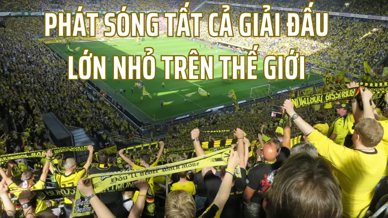
Xoilac TV đặc biệt hiếm hoi tại Việt Nam với việc sở hữu bản quyền phát sóng trực tiếp của toàn bộ các giải bóng đá hàng đầu trong nước và thế giới. Với điều này, chỉ cần truy cập vào website, bạn có thể dễ dàng xem bất kỳ trận đấu nào mà bạn quan tâm một cách đơn giản và miễn phí. Dưới đây là một số giải đấu chính được chúng tôi phát sóng:

Ngoài ra, Xoilac còn phát sóng nhiều giải đấu khác như Nations League, Champions League, Europa League và nhiều giải đấu khác. Tất cả đều được phát sóng trực tiếp và miễn phí trên kênh này, mang lại cho người xem trải nghiệm đầy đủ và chất lượng.
XoilacTV tự hào là kênh trực tiếp bóng đá hàng đầu, sẵn sàng phát sóng tất cả các trận đấu hấp dẫn của Euro 2024 và vòng loại World Cup 2026. Hai giải đấu này là những sự kiện lớn và đặc biệt được quan tâm rất nhiều bởi người hâm mộ bóng đá trên khắp thế giới.
Đây là giải đấu lớn nhất dành cho các đội tuyển quốc gia châu Âu có vé tham dự, quy tụ những đội bóng hàng đầu và các cầu thủ xuất sắc nhất khu vực.
Được tổ chức 4 năm một lần, World Cup là giải đấu cao quý nhất trên thế giới, thu hút sự quan tâm của hàng triệu người hâm mộ và là nơi quy tụ tất cả các đội tuyển mạnh nhất từ khắp châu lục.
Xôi Lạc không chỉ tập trung vào các giải đấu quốc tế mà còn phát sóng toàn bộ các giải đấu quốc nội trong khu vực và đội tuyển Việt Nam tham gia, bao gồm U23 Châu Á, AFF Cup, vòng loại World Cup khu vực Châu Á, Sea Games, và nhiều giải đấu cỏ khác. Điều này giúp đảm bảo rằng người hâm mộ có thể theo dõi tất cả các trận đấu quan trọng và cảm nhận niềm đam mê với trái bóng tròn từ mọi góc cạnh.
Xoilac không chỉ là một trong những trang web phát sóng bóng đá trực tiếp hàng đầu tại Việt Nam, mà còn có những ưu điểm độc đáo và nổi bật so với các trang web khác. Dưới đây là những điểm mạnh chính của Xoilac:
Những đặc điểm này giúp Xôi Lạc TV nổi bật và đáp ứng đầy đủ nhu cầu của cộng đồng người hâm mộ bóng đá.

Để có trải nghiệm xem trực tiếp bóng đá hôm nay tốt nhất tại Xoilac, bạn cần chú ý đến các thông tin và thực hiện một số bước sau:
Kết nối ổn định đường truyền Internet: Bạn phải đảm bảo thiết bị có kết nối Internet ổn định để khi xem phát sóng bóng đá trực tuyến mượt mà, không gặp sự cố lag hay giật.
Xử lý sự cố khi xem bóng đá suốt 90phut: Nếu gặp sự cố như đứng hình, lag, bạn có thể dừng lại 1-2 phút và sau đó nhấn F5 để refresh trang. Điều này giúp khắc phục các vấn đề có thể xuất hiện và xem mà không bị gián đoạn.
Sử dụng các link tructiepbongda dự phòng: Hệ thống Xoilac cung cấp nhiều link dự phòng và các link trực tiếp bóng đá socolive, cakhiatv, rakhoi tv, vebo tv, mitom tv, caheo tv, chaolua tv, demnay tv, luongson tv, vaoroi tv… để giảm tải cho đường link chính. Bạn có thể chuyển đổi sang các link này nếu gặp vấn đề với đường link chính.
Thưởng thức bình luận viên nhiệt huyết: Đội ngũ bình luận viên của Xoilac luôn nhiệt huyết và truyền cảm hứng, đam mê của họ vào trận đấu. Mời bạn rủ thêm bạn bè, người thân để cùng thưởng thức không khí xem đá bóng tốt nhất.
Đội ngũ vận hành của Xoilac TV cam kết đáp ứng niềm đam mê bằng cách phát sóng trực tiếp bóng đá hôm nay miễn phí cho mọi người, tạo điều kiện cho Fan hâm mộ gần xa có thể tận hưởng không khí tuyệt vời nhất của môn thể thao vua, thông qua trải nghiệm xem bóng đá online. Xôi Lạc TV Tructiepbongda mong rằng mọi người sẽ cùng chia sẻ niềm đam mê cuốn hút, phấn khích, và về bờ thành công qua những trận đấu hấp dẫn trên Xoilac.